SolveInverseProblemWithTikhonov
SolveInverseProblemWithTikhonov solves the inverse problem as a (weighted) minimum norm problem by applying a Tikhonov L2-norm regularization. It solves the minimization problem:
\(\hat{x}=argmin_x \|Ax -Ly\|^{2}_ {2} + \lambda\|Rx\|^{2}_ {2}\)
Detailed Description
The module has four inputs, three outputs, and a graphical user interface (UI) where the regularization parameter can be chosen or computed. All inputs can be generated by SCIRun, or created elsewhere or loaded from Matlab files or the Matlab interface.
Input
Forward problem matrix, \(A\): This matrix describes the relationship between solution and measured signals \(A x = y\). For example, this matrix can be computed by solving the forward problem e.g. using finite or boundary element methods (see modules in BioPSE Forward, FiniteElements category).
Solution constraint matrix, \(R\): This matrix is used to constrain the solution. It imposes some a priori knowledge upon the minimization problem to select solutions with specific properties (expressed as a solution covariance e.g. to achieve maximally smooth solutions). If no input is given the identity matrix will be used.
Data vector, \(y\): These are the measurement data which have to be provided as matrix which should only contain one column.
In case of having a time series (multiple columns), it is recommended to use the module SelectSubMatrix to iterate over the different time instances (columns). In more detail, for each time instance, SelectSubMatrix would provide the data of the current time instance for SolveInverseProblemWithTikhonov to perform an estimation of the inverse solution.Residual constraint matrix, \(L\): This matrix is used to weight the measurements (e.g. by an inverse covariance matrix of the measurement channels). If no input is given, the identity matrix will be used.
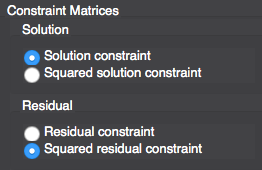
IMPORTANT: Both, residual constraint as well as the solution constraint matrix can be used in single matrix form (such as \(L\) and \(R\)) in the minimization problem or as a squared matrix version (such as \(L^T L\) and \(R^T R\)) respectively. This option must be properly selected by the user in the UI:
Output
Inverse solution, \(\hat{x}\): computed solution estimate.
Regularization parameter, \(\lambda\): used regularization parameter.
Regularized inverse matrix, \(G\): linear inverse operator that gives a solution estimate equation \(\hat{x} = G y\). It actual value depends on the selected formulation (underdetermined or overdetermined) and requires the inversion of a matrix. It is only calculated if this port is connected to another module’s input port. The user can select between the formulations using the module GUI (see section Computation).
underdetermined:
\(G=RR^TA^T (ARR^TA^T + \lambda LL^T)^{-1}\)
overdetermined:
\(G=(A^TL^TLA + \lambda R^TR)^{-1}A^TL^TL\)
Computation
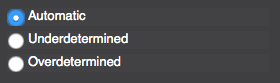
The algorithm has two different ways of computing the solution: the underdetermined and the overdetermined formulations. To choose which one will be solved the module has three options:
Automatic selection. The algorithm will select underdetermined or overdetermined based on the dimensions of the Forward matrix.
Manual selection of the undetermined formulation.
Manual selection of the overdetermined formulation.
These options are presented in the GUI as follows:
Both cases use Gaussian elimination to calculate the unknown \(\hat{x}\), but they differ in the equations to solve for:
underdetermined:
\((A R R^T A^T + \lambda L L^T) b = y, \hat{x} = R R^T A^T b\)
overdetermined:
\((A^T L^T L A + \lambda R^T R) \hat{x} = A^T L^T L y\)
However, If the output port of the inverse operator is connected to another module’s input the inverse operator \(G\) is used to compute the solution estimate \(\hat{x}\) such as \(\hat{x} = G y\).
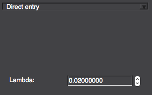
In both cases the used regularization parameter can be chosen in the UI. The available options are:
Fix \(\lambda\) manually.
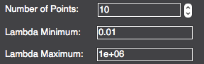
Automatic selection of \(\lambda\): the corner of the L-curve is determined by maximal curvature. A number of regularization parameter points (different \(\lambda\) values) can be specified in the L-curve plot which are than equally distributed over the range (“Lambda Range”, see below) of \(\lambda\)’s to be used in the L-curve computation.
Fix \(\lambda\) manually based on the range of regularization parameters (\(\lambda\)) specified by the “Lambda Range” input.
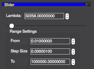
For the options that use the L-curve, the user can define the range and step size in the UI: