Classic Tutorial
Overview
SCIRun is a modular dataflow programming Problem Solving Environment (PSE). SCIRun has a set of Modules that perform specific functions on a data stream. In SCIRun, a module is represented by a rectangular box on the Network Editor canvas. Each module reads data from its input ports, calculates the data, and sends new data from output ports. Data flowing between modules is represented by pipes connecting the modules. A group of connected modules is called a Dataflow Network (see Fig. 32), and are saved as .srn5 files. Any number of nets can be created, each solving a separate problem.
This tutorial demonstrates the use of SCIRun to visualize a tetrahedral mesh and the construction of a network comprised of three standard modules: ReadField, ShowField, and ViewScene. This tutorial also instructs the user on reading Field data from a file, setting rendering properties for the nodes, edges, and faces (the nodes are rendered as blue spheres), and rendering geometry to the screen in an interactive ViewScene window).
Software requirements
SCIRun
SCIRun is available for download on the GitHub release page. Make sure to update to the most up-to-date release available, which will include the latest bug fixes. Use the supplied installers to install SCIRun on your local machine. Linux users may have to build from source.
Download the SCIRunData file as a zip or tgz. Unpack it in a convenient location, then add the base directory to the SCIRun Data Path in the SCIRun preference window, under the Paths tab (Fig. 30)
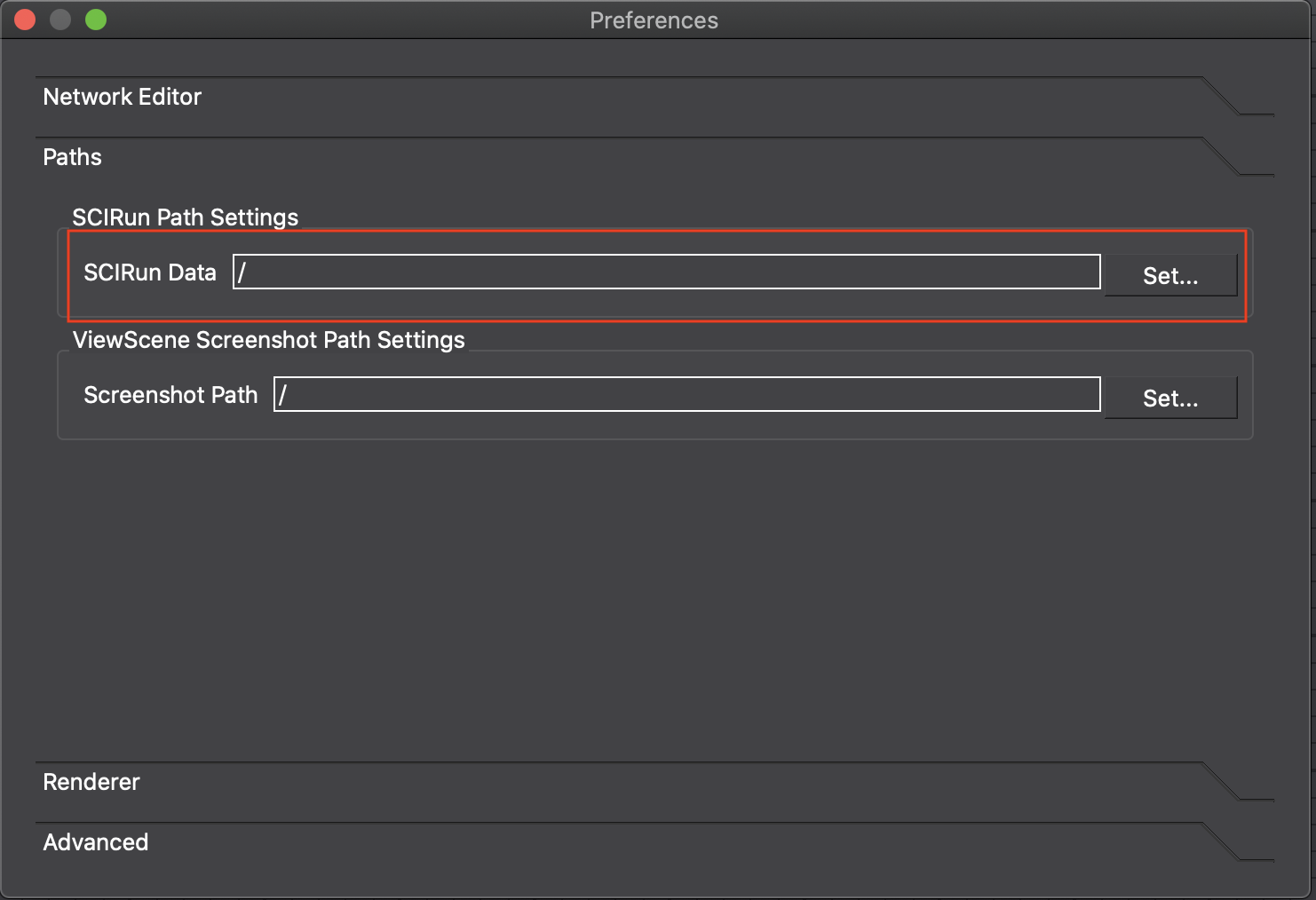
Fig. 30 The the Paths tab of the SCIRun preference window.
Starting SCIRun
To open the main SCIRun window, launch SCIRun by either double clicking on the binary icon or by launching SCIRun from the command line. Once SCIRun has been launched, the main SCIRun network editor will appear (Fig. 31).
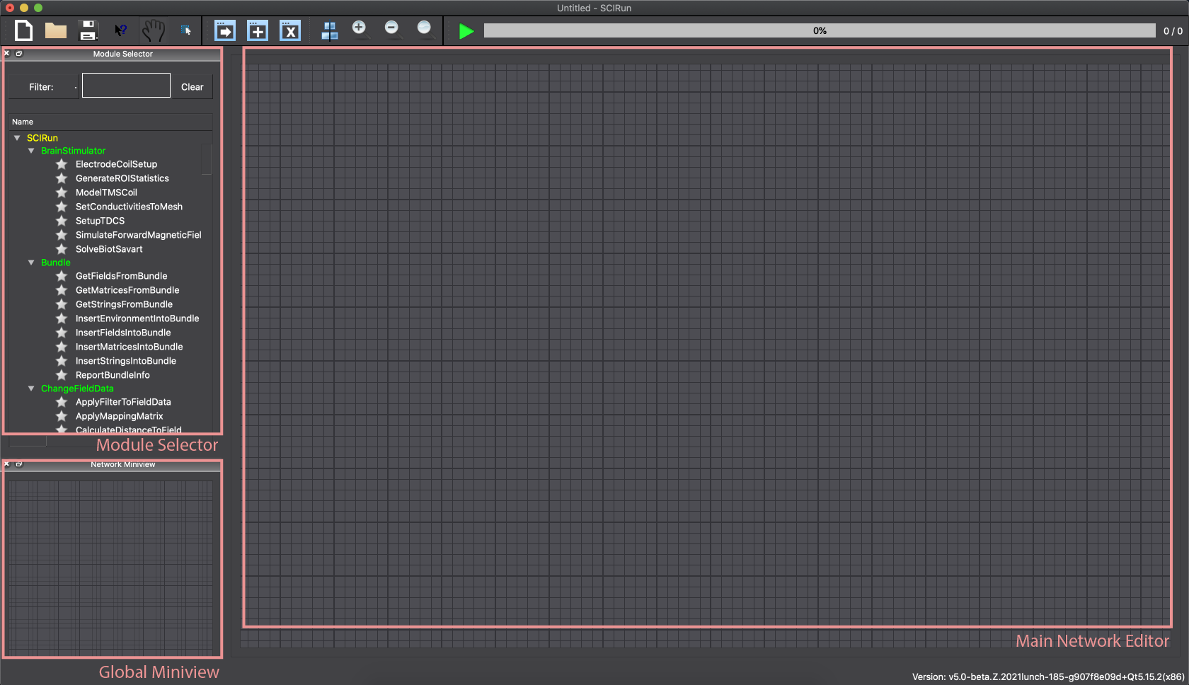
Fig. 31 The main SCIRun window and components
SCIRun Network Building Blocks: Modules and Connections
Lets begin constructing the network pictured in (Fig. 32). (Note: subsequent tutorial chapters expand on this network, adding more features and functionality.) This network loads a geometric mesh from a data file and renders it to the screen.
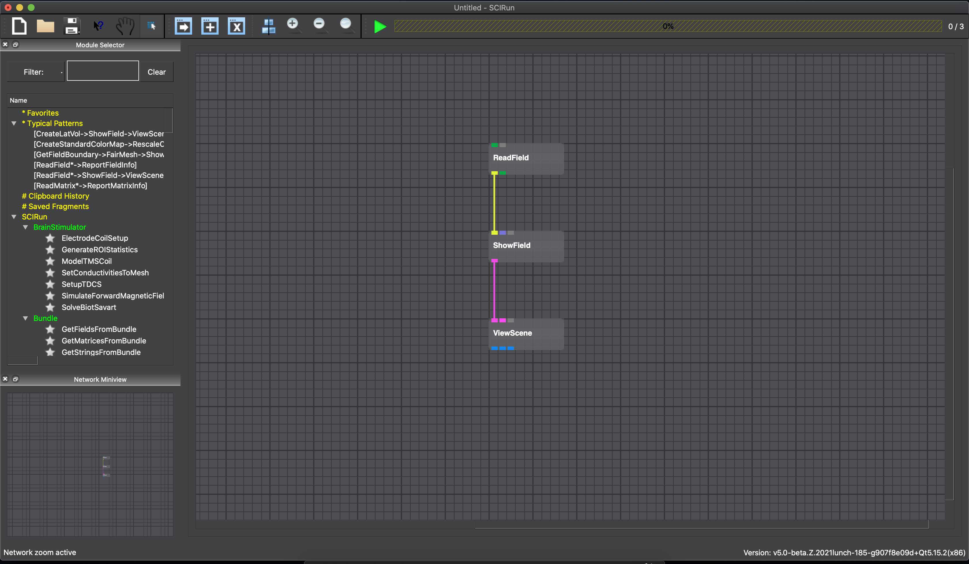
Fig. 32 Network editor after building example network
Modules: A module is a single-purpose unit that functions within a dataflow environment. Modules have at least one input port for receiving data, located at the top of the module, or one output port for sending data, located at the bottom of the module (Fig. 33).
All modules have an indicator that alerts the user to messages that exist in a module’s log. Different colors represent different types of messages. Gray means no message, blue represents a Remark, yellow a Warning, and red an Error. To read messages, click the module’s indicator button to open the log window.
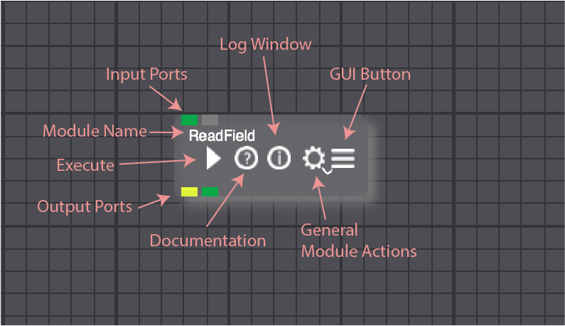
Fig. 33 SCIRun Module icon
Pipes: Data is transferred from one module to another using dataflow connections, commonly referred to as Pipes. Each dataflow pipe transfers a specific datatype in SCIRun, denoted by a unique color. Pipes run from the output Port of one module to the input Port(s) of one or more other modules. Ports of the same color correspond to the same datatype and can be connected.
Two or more connected modules form a SCIRun network.
ReadField Module
Now it is time to begin creating a SCIRun network. First, create a ReadField module, which will be used to load a SCIRun Field dataset from disk.
Select ReadField under the DataIO section in the module selector located on the left side the the main SCIRun window, as show in (Fig. 34).
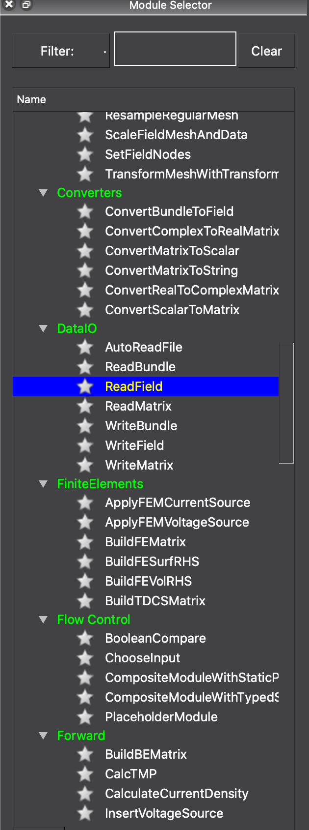
Fig. 34 Module creation (ReadField)
The ReadField module will appear on the NetEdit frame. Now, set user interface parameters for this module, by pressing the UI button on the module. This brings up a standard file selection dialog (Fig. 35). Select the utahtorso-lowres/utahtorso-lowres-voltage.tvd.fld input file. (Note: This file can be found in the SCIRunData directory. This directory should have been downloaded and installed when SCIRun was installed.) This dataset contains a low resolution tetrahedral mesh of a human torso.
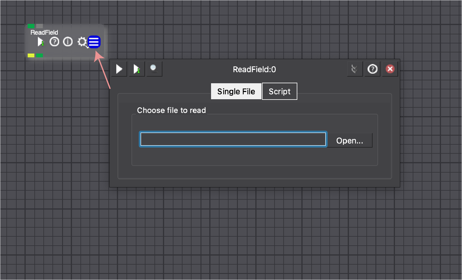
Fig. 35 ReadField file selection GUI
Once the file has been selected, the following will occur:
The file selection window disappears.
The module reads in the dataset (a SCIRun Field) and the progress bar turns green.
Brief Field Overview
A Field contains a geometric mesh, and a collection of data values mapped on to the mesh. Data can be stored at the nodes, edges, faces, and/or cells of the mesh. In this case, a tetrahedral mesh with voltages defined at the nodes of the mesh has been selected.
The dimensionality of the mesh type determines the available storage locations. For example, a TriSurf mesh has nodes, edges, and planar faces, but not cells, which are assumed to be three-dimensional elements. As a result, a TriSurf cannot store data in cells, but can store data in edges or faces.
See Appendix 1 for a description of various types of geometric meshes, data values, and mappings SCIRun supports.
Hooking Modules Together
Now add a second module to the network. This module is used to visualize various Field types. Then connect the two modules in the canvas so data can flow between them.
Create a ShowField module using the DataIO section in the module selector (use the same menus used to create the ReadField module).
Position the mouse pointer over the yellow output port on the ReadField. Press and hold the left mouse button. The name of the port and lines indicating possible data pipe connections will appear.
Continue to hold the left mouse button and drag the mouse toward the first yellow ShowField input port.
The line turns red, showing the desired connection has been selected. See (Fig. 36).
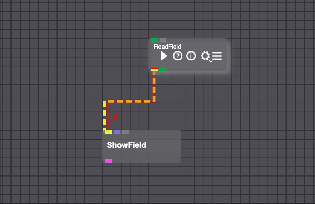
Fig. 36 Pipe Selection Options
Release the mouse button. A yellow pipe showing a data flow connection between ReadField and ShowField will appear (Fig. 37).
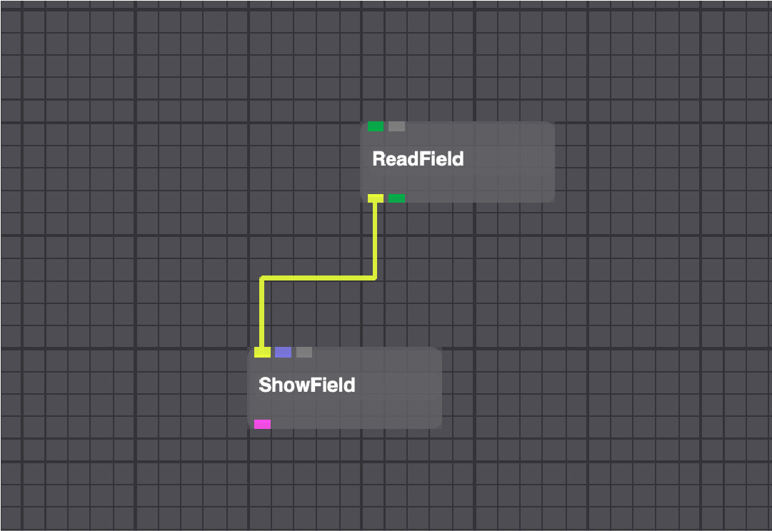
Fig. 37 Connected Dataflow Pipe
Setting the ShowField User INTERFACE_MODULES_
The ShowField module has options for changing the visual representations of a Field’s geometry. To illustrate the module’s functionality, change ShowField parameters using its GUI (found by clicking the GUI button on the ShowField module (Fig. 33)). Specifically, change the color of the nodes to blue spheres.
Select the UI button on the ShowField module.
Select the Default Color button near the top of the GUI to change the default color and a separate Color Chooser GUI appears.
In the Color Chooser GUI, use the sliders to adjust the color values. Select a blue color.
Select the OK button in the Color Chooser GUI. Notice that the Default Color swatch in the ShowField GUI has changed to blue. SCIRun and the ShowField GUI should now look like Fig. 38.
Close the Color Chooser GUI.
Set the name of the Field to Voltage. This makes it easy to identify the Field in the ViewScene Window (discussed later).
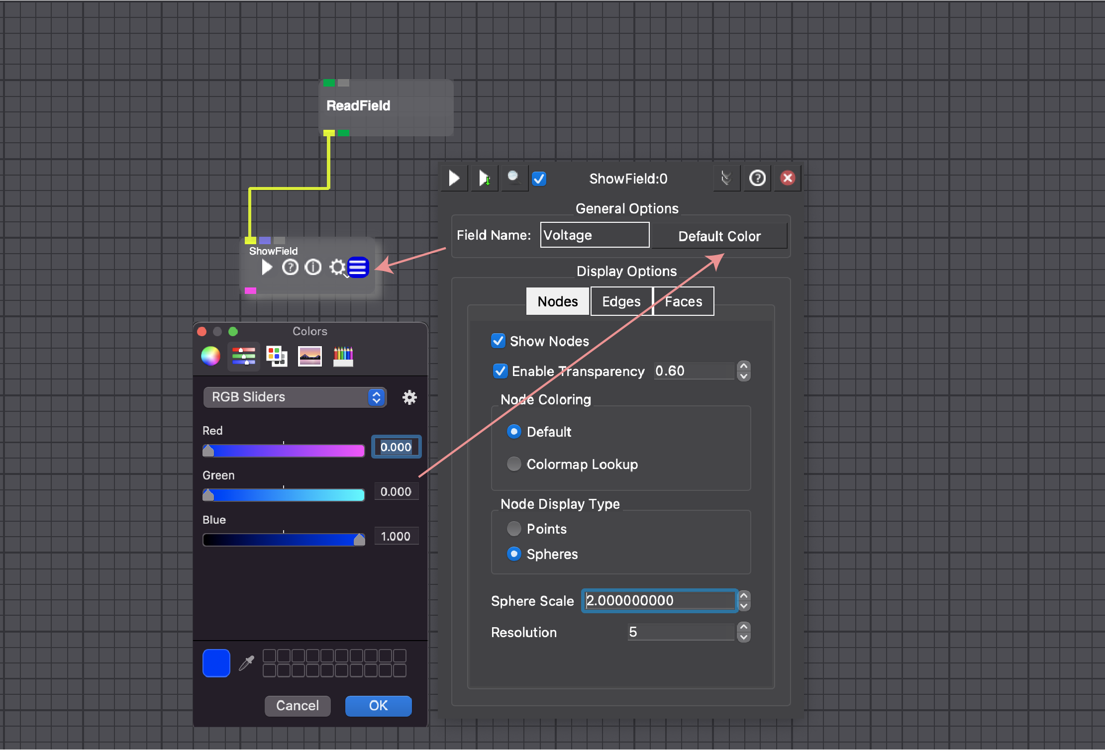
Fig. 38 ShowField GUI
Now change the scale and resolution of the nodes.
In the ShowField GUI, a spin box widget represents the Node Scale. The Node Scale interval can be increased or decreased by a power of 10 by pressing the up and down arrows. Set the Scale to 2. Make sure the Node Display Type is set to Spheres.
Set the Sphere Resolution to 5.
Go to the Edges tab and turn off the display of edges by deselecting the Show Edges check box.
Go the the Faces tab and repeat the same action.
Close the ShowField GUI by pressing the Close button.
The ShowField module is ready to render the nodes as blue spheres. The module Interactively Updates, by default, to execute after every user GUI change. Users can select the Execute button only box to delay all changes until the Execute button is pressed. (This is useful with large dataset, when rendering takes a long time.)
ViewScene modules
The ViewScene is the last module that will be added to the network.
Create a ViewScene module by selecting the module under the Render section in the module selector.
Connect the output port from ShowField into the ViewScene input port. Notice the ViewScene module automatically creates a new input port; this is an example of a SCIRun module that has dynamic input ports. This allows the ViewScene module to support an infinite number of geometry producing modules.
Open the ViewScene window by pressing the ViewScene’s UI button.
In the ViewScene window, there is a set of axes, representing X, Y, and Z directions. To make all of geometry piped to the viewer visible, press the Autoview button located on the top menu of the window. (Note: any time the view is changed (scaled, rotated, or translated), and you want the viewer to re-display everything in the center of the screen, use the Autoview button.) At this point, the utah-torso voltage Field should appear in the ViewScene window. It should appear similar to Fig. 39, but will be somewhat different as the figure has been scaled and rotated.
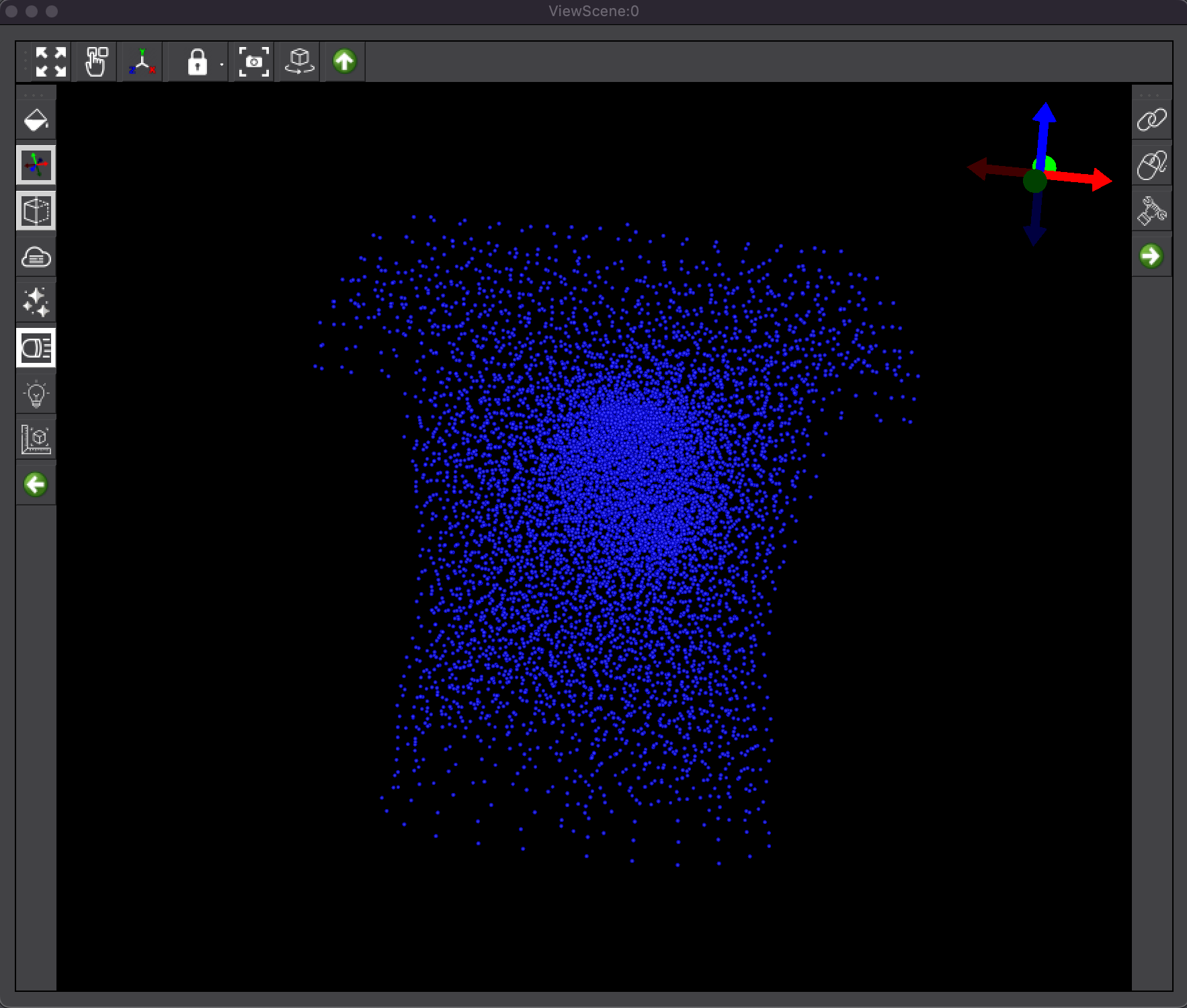
Fig. 39 ViewScene window showing the utahtorso-lowres-voltage data
Mouse Controls
In the Viewer, the mouse can be used to rotate, scale, and translate the image.
Scaling the scene (Scroll Wheel)
Scroll up to zoom the image out.
Scroll down to zoom the image in.
Setting Visualization Parameters
Now review the tools at the top of the ViewScene window (see Fig. 40). Buttons at the top of the ViewScene window are used for the following functions (for detailed information about the functionality of each tool, refer to the ViewScene module documentation):
Auto View: restores the display back to a default condition. This is very useful when objects disappear from the view window due to a combination of settings
Object Selection
View Options
Camera Locks
Screenshot
Auto Rotate
Buttons on the left side of the ViewScene window (see Fig. 40) are used for the following functions:
Background Color
Orientation Axes
Plane Settings
Fog Controls
Material Properties
Headlight
Additional Lights
Scale Bar
Buttons on the right side of the ViewScene window (see Fig. 40) are used for the following functions:
Groups
Mouse Controls
Report Problems
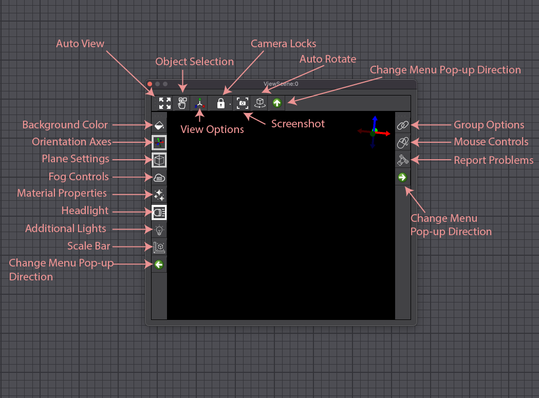
Fig. 40 ViewScene window controls
Saving and reloading networks
Now that a three-module network has been created, save it to disk. The .srn5 file can easily be reloaded in a future SCIRun session.
Saving a SCIRun network:
Click on the File menu (at the top of the Network Editor window) and select “Save As.”
When the file browser appears, follow the prompt to choose a location and filename for the network. Many example networks are stored in the ExampleNets directory, which is distributed with the binaries, or in SCIRun/src/ExampleNets. The network can be stored in any location with write access.
For this example, store the net as SCIRun/src/nets/show-torso-mesh.srn5, as in Fig. 41. The .srn5 suffix is used for SCIRun network files
Please note, to avoid losing work, it is strongly recommended that nets be saved frequently. Auto-save can also be enabled in the SCIRun Preferences window.
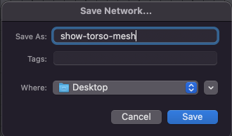
Fig. 41 “Save As” GUI
Click the Save button. The network is saved, and the dialog disappears.
Exit SCIRun by closing the main SCIRun window or pressing Ctrl-Q.
Loading a SCIRun network:
Start SCIRun.
From the File drop-down menu, select the the Load… option.
Select the previously saved net (SCIRun/src/nets/show-torso-mesh.srn5).
The net reloads into SCIRun, where it was previously saved. If the net was saved with any of the module UIs open, those UIs automatically re-open when loaded to the net. After changing module settings (e.g., rotating the image in the ViewWindow or changing the rendering color of the nodes in ShowField), there are two options for re-saving the net:
Overwrite existing show-torso-mesh.srn5 file by using File->Save from the drop-down menu.
Save the net to a new file by using File->Save As…
Appendix 1
SCIRun has nine geometric meshes available for Fields:
 PointCloudMesh: unconnected points
 ScanlineMesh: regularly segmented straight line (a regular 1D grid)
 CurveMesh: segmented curve
 ImageMesh: regular 2D grid (see note below)
 Structured Quad Surface mesh: surface made of connected quadrilaterals on a structured grid
 Structured Hex Volume mesh: subdivision of space into structured hexagonal elements
 TriSurfMesh: surface made of connected triangles
 QuadSurfMesh: surface made of connected quadrilaterals
 LatVolMesh: regular 3D grid
 TetVolMesh: subdivision of space into tetrahedral elements
 HexVolMesh: subdivision of space into hexagonal elements
 PrismVolMesh: five faces, two triangular faces connected together by three quadrilateral faces.
The following data types can be stored in a Field:
tensor
vector
double precision
floating point
integer
short integer
char
unsigned integer
unsigned short integer
unsigned char